Lane Detection in Images
Our first goal of this project was to detect lanes in images. This was the most complicated part of our project, and laid the groundwork for video lane detection and stop sign detection. To approach this problem, we read several articles on the best practices in lane detection coding, specifically "A Real-Time System for Lane Detection Based on FPGA and DSP" and "Lane Detection Based on Connection of Various Feature Extraction Methods," which can be found on our citations page.
In order to get the most accurate results possible, we used two different methods to detect lanes. In Method 1, we developed our own Canny edge detector, and used the Roberts gradient intensity calculator within that detector. In the second method, we implemented the built-in MATLAB Canny edge detector, but used different pre-processing methods on our images, such as the Gaussian blur and the built-in bwareaopen MATLAB function.
Finally we combined these two methods using our developed slope calculator. The goal of this was to combine our two methods to get the best possible results.
Each of these methods and our unique slope combination methodology is described in the sections below.
Method 1
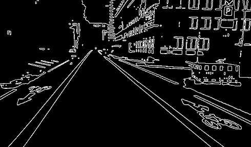
In our first lane detection method, we developed our own Canny edge detector by performing the known steps of the Canny Method: Gaussian blurring, intensity gradient calculation, non-maximum suppression, and linking discontinuous edges. Our method is derived from IEEE studies, which can be found in our citations section.
The first step of our method is convert the image to HSV, then we used both the Otsu Method and Roberts operator to outline all of the potential lanes in our image. Finally we used the built-in Hough Transform to outline the lanes in our images.
This process is described in more detail below.

Step 1: HSV
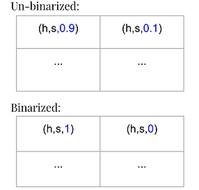
The first step is converting the image to HSV, and converting it from a colored image to a binarized logical image. To do this, we set every value between 0 and 0.65 to 0, and any value greater than 0.65 to 1.
Step 2: Otsu Method
The pre-processing step for the Otsu method is grayscale conversion. After that step, the Otsu algorithm determines an intensity threshold that separates pixels into either foreground or background where the foreground will be binarized to a logical 1 and background is a logical 0. According to the Otsu IEEE study the threshold is determined by maximizing inter-class variance of a grayscale histogram.

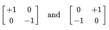
As mentioned on the 'Theory' page, the Roberts operator is a gradient intensity calculator. It works by convolving two kernels with an image, and its overall purpose is to detect edges. The horizontal (left) and vertical (right) kernels for this operator are shown below.
As mentioned on the 'Theory' page, the Hough Transform is used to join disconnected pixels to create continuous lines. This section also parametrizes the detected lines so that they can be plotted on the image.
Method 2
In addition to our personalized Canny detector, we wanted to try the built-in MATLAB Canny function. To customize the output of the MATLAB function, we implemented several pre-processing techniques that were listed as best-found practices in various IEEE studies.
We will go into more detail of this method below.
As mentioned on the 'Theory' page, the Gaussian Blur is a method of blurring and smoothing an image by convolving that image with a Gaussian function. The convolution acts as a low-pass filter, and reduces noise by eliminating higher frequency components.

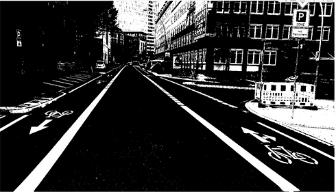
Step 2: Binarization
The image was binarized into a logic image using the RGB values of the images' pixels. If the red green and blue values in all 3 channels are above a threshold of 130, then the pixel would be set to 1 in the binarized version of the original image, otherwise, the value would be set to 0.

Step 3: Canny Operator
In this section, edges are detected by finding local maxima of the image gradient. This functions calculates and uses two thresholds, one to detect prominent edges and another for weak edges. The multiple threshold method allows the Canny edge detector to differentiate noise from straight lines.
Step 4: Noise Removal
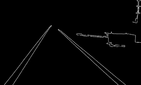
In this step all of the connected components or points that have fewer than a threshold number of pixels are eliminate. This process creates another binary image that filters out noise and only focuses on larger and more important features of an image. This step is performed by the MATLAB function bwareaopen.
As mentioned on the 'Theory' page, the Hough Transform is used to join disconnected pixels to create continuous lines. This section also parametrizes the detected lines so that they can be plotted on the image.
Analysis of Our Methods
As mentioned before, the reason we used two methods to detect lanes was to increase our accuracy. When used individually, Method 1 and Method 2 are only able to detect small segments of lanes, instead of detecting the full length of the lanes.
The two methods differ in which lines they detect because they utilize different pre-processing techniques. For the first method, we filtered the image based on a threshold value applied to an HSV image, converted the image to grayscale, used Otsu method binarization, and convolved with a Roberts edge detector.
For the second method, we created a binary image based on a threshold value applied to all 3 channels of the RGB version of the picture. Unlike the last method, we directly applied MATLAB’s Canny edge detector and used additional built in MATLAB functions, like bwareaopen(BW,P), to filter out non-essential information in the picture.
The differences in these processes cause each method to detect a different light intensity, which leads to them detecting different segments of the lame line.
Our Own Algorithm
Due to the different pre-processing and edge detection procedures we used in our methods, each method was detecting different portions of the same line segment rather than the whole line segment itself.
To optimize our lane detection program, we created our own algorithm to combine Methods 1 and 2. We achieved this by finding discrepancies between detected lines and essentially filling in these gaps.
To implement this algorithm, we used the concepts of equivalent slopes, permutations, and maximum distances, which are described below.
Step 1: Find Equal Slopes
First, our algorithm checks the slopes of each identified line segment outputted from each method. If a line segment from Method 1 has the same slope as a line segment from Method 2, these segments are assumed to be a part of the same line (same slope = same line).
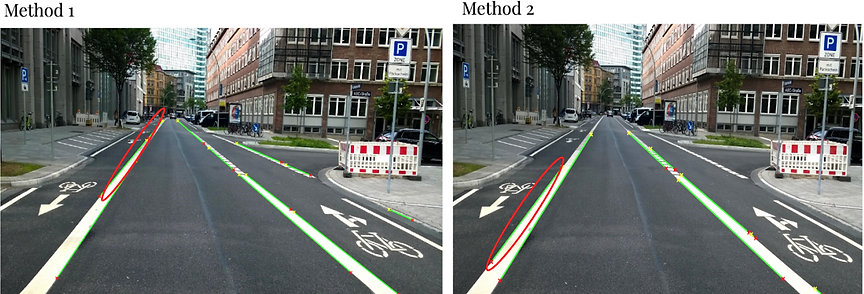
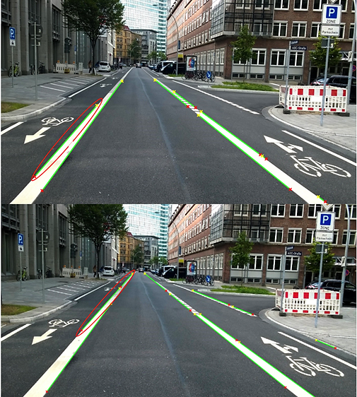
Looking at the bottom portion of the image on the left, we see all the line segments outputted from Method 2, with the top image corresponding to Method 1.
The red circles on the images indicate examples of lines detected by Method 1 and Method 2. Our algorithm is then able to recognize these segments as having equivalent slopes. Hence, the program considers these segments to be part of the same line.

Step 2: Maximum Distance Permutations
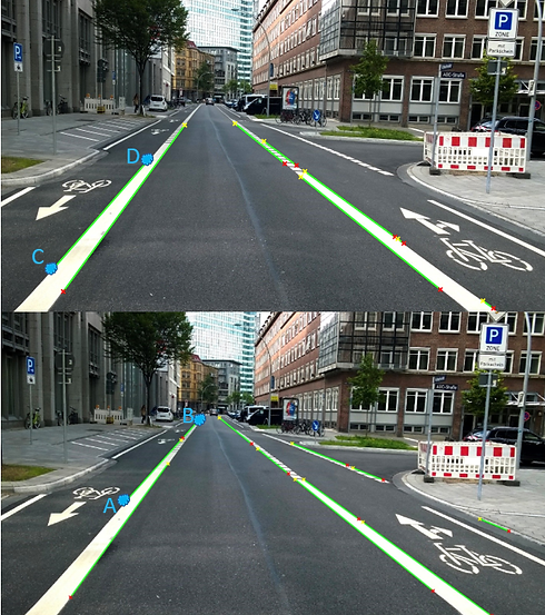
After finding a pair of line segments with equivalent slopes, our algorithm calculates the distance between each possible permutation of end points (4 points total, 6 possible combinations of two points).
The pair of points that corresponds to the maximum distance is the new start and end point of our algorithm's final plotted line.
For the example on the right, the maximum distance occurs with start point C, and an end point B.
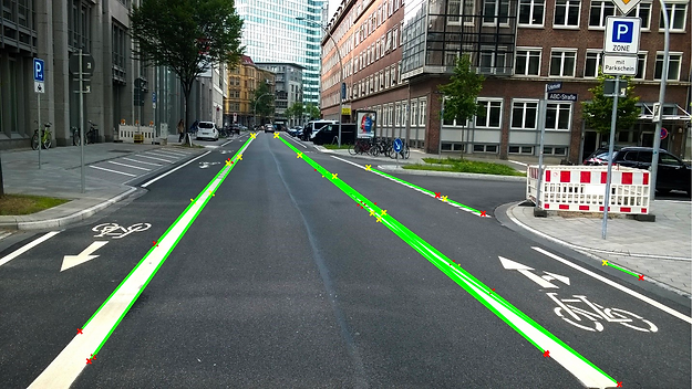
Our Algorithm's Final Result
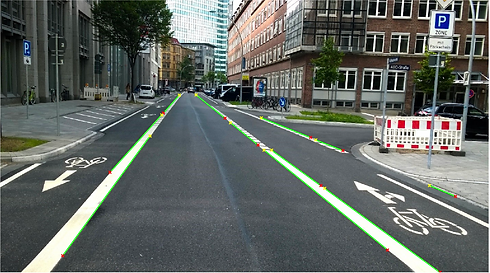
Additional Test Cases
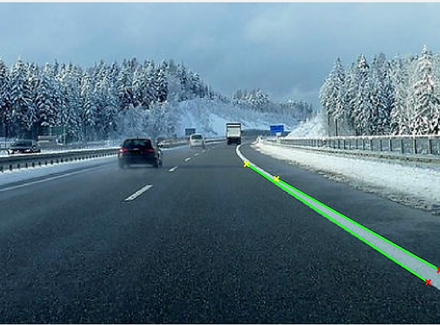
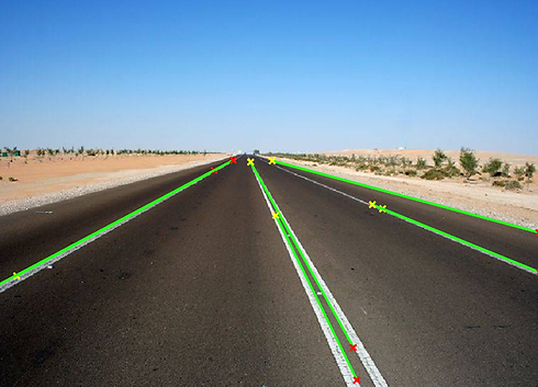
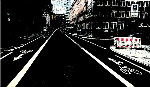
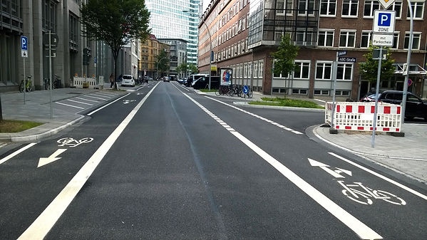
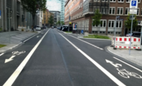
These are some examples of resulting images when run with our algorithm. In the image to the right, we see our algorithm works very well with straight lanes. To the lower right, we see that even in crowded areas with obstacles, our algorithm is still quite accurate and able to detect the lanes. The image below shows our algorithm is even able to detect white lanes in a white, snow-covered environment.